Data Validation lists are drop-down lists in a cell that make it easy for users to input data. If you’ve never worked with data validation lists before, I suggest you start with this tutorial for creating drop-down lists in cells before moving on.

In today’s post, I want to show you how to make your drop-down list dynamic.  In other words, your list can automatically be updated with new options when you add or subtract entries to your source range.

This is done in three simple steps:

I’ll explain in more detail below.

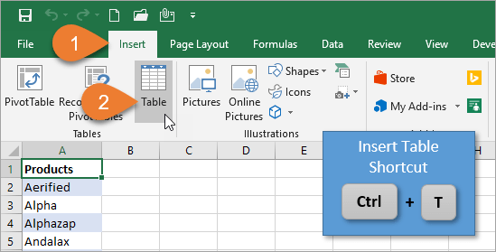
To begin, we will format our source range to be an Excel Table. On the Insert tab, you’ll chose the Table button.  The keyboard shortcut for inserting a Table is Ctrl+T.

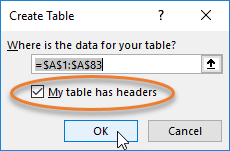
The Create Table window will appear, showing the range of cells that will be in your Table.  Since our column begins with a header (“Products”), we want to make sure the checkbox that says “My table has headers” is checked. If we don’t check that box, the column title will be included in our source range and will appear as one of the options in our drop-down list.

If you haven’t used Tables before, I recommend checking out my Excel Tables Tutorial Video.